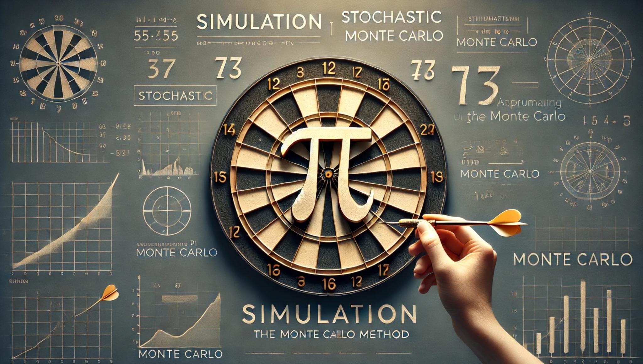
Stochastic Simulation & The Monte Carlo Method

Imagine you’re trying to predict the outcome of a situation with many unknowns—like how much a beam might bend under load, or how marine structures will hold up against unpredictable waves and currents. This is where stochastic simulation becomes invaluable.

Stochastic simulation allows us to explore and understand systems that have inherent randomness or uncertainty. Instead of producing a single, fixed outcome, this approach considers multiple possibilities, helping us predict what might happen across a range of scenarios. Think of it as rolling a dice multiple times to see the variety of results, then using that information to make informed decisions.

The Monte Carlo Method: A Versatile Tool

The Monte Carlo method is one of the most widely used techniques in stochastic simulation. Named after the famous Monte Carlo Casino—where chance rules the day—this method leverages random sampling to solve problems that are deterministic in theory but too complex to tackle directly. By performing a large number of simulations with different inputs, it allows us to estimate probabilities and make well-informed decisions.

Example: Approximating Pi

Let’s start with a fun and simple example: approximating the value of π (Pi). π is a fundamental constant in mathematics and engineering, especially in calculations involving circles. But what if we could approximate it not by measurement or a complex formula, but by harnessing the power of randomness?

How It Works

1. Visualise The Problem

Imagine a square dartboard with a circle perfectly inscribed within it. The square has side lengths of 2 units (from -1 to 1 on both the x and y axes), and the circle has a radius of 1 unit.

The area of the square is 4, and the area of the circle is π.

2. Simulate Dart Throws:

Randomly generate points within the square. Each point represents a dart throw.

Determine if the dart lands inside the circle by checking if the point satisfies the equation

3. Calculate π:

By counting the number of darts that fall inside the circle and comparing it to the total number of darts thrown, you can estimate the value of π using the formula

Try It Yourself: Python Script for Approximating Pi

Here’s a simple Python script that lets you simulate this process and see how close you can get to the true value of π:

import random

import math


def throw_darts(num_darts):

    inside_circle = 0

 
    for _ in range(num_darts):

        # Generate random (x, y) point

        x = random.uniform(-1, 1)

        y = random.uniform(-1, 1)

 
        # Check if the dart is inside the circle

        if x**2 + y**2 <= 1:

            inside_circle += 1

 
    # Estimate π

    pi_estimate = 4 * (inside_circle  num_darts

     pi_estimate

 
 

    

       

     

        

            num_darts  

             num_darts  

                 ValueError

            

         ValueError

            

 
    

    pi_estimate  throw_dartsnum_darts

    

    

    

 

 __name__  

    main
    

Running the Script on Your Desktop

Install Python:

If you don’t have Python installed, you can download it from python.org. Make sure to check the box to add Python to your system PATH during installation.

Save The Script

Copy the script above into a text editor and save it with a .py extension, like approximate_pi.py.

Run the Script:

Open Command Prompt (search for cmd in the Windows Start menu).

Navigate to the directory where you saved the script using the cd command.

Type python approximate_pi.py and hit Enter.

Follow the Prompts: The script will ask you how many darts you want to throw. The more darts, the more accurate your approximation will be.

The Results

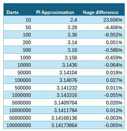
To further explore the effectiveness of the Monte Carlo method in approximating the value of π, we conducted a series of simulations, increasing the number of dart throws—or random points generated—with each iteration. The table below summarises the results, showing how the accuracy of the π approximation improves as more darts are thrown.

Observations from the Results

As seen in the table, when only 10 darts were used, the π approximation was quite poor, with a value of 2.4 and a percentage difference of over 23% from the actual value of π (3.14159…). This is expected due to the very small sample size, where randomness can cause significant deviations from the true value.

However, as the number of darts increases, the approximation rapidly improves. By the time we reach 1,000 darts, the approximation is 3.156, with the percentage difference dropping to -0.459%. This trend continues as we scale up the number of darts. With 1,000,000 darts, the approximation stabilises around 3.141316, with a minimal percentage difference of -0.055%.

At 10,000,000 darts, the approximation is impressively accurate at 3.14173864, differing from the actual value by just -0.005%. These results clearly demonstrate the power of the Monte Carlo method: with enough random samples, even a process that relies purely on randomness can yield highly accurate results.

What This Means

This experiment highlights how the Monte Carlo method’s accuracy improves with larger sample sizes. Initially, with fewer darts, the randomness leads to more significant errors. But as the number of darts increases, the law of large numbers comes into play, averaging out the random errors and honing in on the true value of π.

These findings are not only a testament to the power of stochastic simulation but also serve as a practical reminder of the importance of sample size in any Monte Carlo analysis. Whether you’re using this method to approximate π or to predict the behaviour of complex engineering systems, the principle remains the same: more data points lead to more accurate predictions.

Conclusion

Stochastic simulation, with tools like the Monte Carlo method, offers us incredible insights into systems with inherent uncertainty—whether it’s predicting how much a beam might bend under load, ensuring the safety of offshore structures, or finding creative ways to approximate π. By embracing the power of randomness, engineers can design safer structures, optimise performance, and tackle complex problems that would otherwise be too daunting to solve.

So, whether you’re simulating beam deflections, evaluating the stability of marine structures, or just having fun with dart throws, stochastic simulation is a fascinating way to explore the unpredictable and make better decisions based on what you discover. Give it a try, and see the power of randomness in action!

Other Engineering Applications of the Monte Carlo Method

The Monte Carlo method isn’t just a mathematical curiosity; it’s a powerful tool with real-world engineering applications, especially in fields where uncertainty and variability play a significant role.

1. Cantilever Beam Deflection

Consider a cantilever beam—a beam fixed at one end and free at the other—used in construction or mechanical systems. The beam is designed with specific dimensions and material properties, but due to manufacturing processes, there are always slight variations in length, width, height, and material strength. These variations can affect how much the beam will deflect (bend) when a load is applied to its free end.

Using stochastic simulation, we can model these variations as random variables and simulate how the beam will behave. By feeding these variables into the deflection formula for a cantilever beam, we can run thousands of simulations to see the range of possible deflections. The result is a probability density distribution that tells us not just what the beam’s deflection might be, but what it’s most likely to be. This information is crucial for engineers who need to ensure that structures remain safe and functional under all possible conditions.

2. Marine Engineering: Waves and Currents

In marine engineering, the Monte Carlo method is invaluable for analysing how offshore structures, such as oil platforms or wind turbines, will withstand the unpredictable forces of waves and currents. The ocean is a dynamic environment, and the loads exerted on structures can vary dramatically depending on wave height, frequency, direction, and current speed.

By simulating a wide range of wave and current conditions using random variables, engineers can predict the likely range of forces that a structure will experience over its lifetime. This helps in designing more robust and resilient structures, ensuring they can endure even the most extreme sea states. For instance, engineers can use Monte Carlo simulations to assess the probability of a platform’s failure or the wear and tear on subsea cables, leading to better maintenance planning and safer operations