Matrices in engineering: how they work and what they solve
Almost every engineering calculation ends in the same place: a handful of unknowns tied together by a handful of equations. The reactions under a skid, the tensions in four lifting slings, the stresses at a weld toe, the displacements of every node in a finite element model. Matrices are how engineers write those equations down so they can be solved, checked and repeated, whether there are two unknowns or two million.
This lesson builds up from the simplest case, a plank on two props, to the stiffness matrix at the heart of finite element analysis (FEA). Along the way it covers the few matrix operations that do almost all the work, and the checks that tell you whether to trust the answer. It is based on one of our internal lunch and learn sessions.
What a matrix is
A matrix is a rectangular table of numbers, described by its rows and columns: a 2 × 3 matrix has two rows and three columns. A matrix with a single column is called a vector. In engineering the rule that makes matrices useful is simple: each row is one equation, and each column is one unknown. The number in row i and column j says how much unknown j contributes to equation i.
Multiplying a matrix by a vector works row by row: go across the row and down the vector, multiply the pairs and add them up. That one operation turns a set of simultaneous equations into the compact form A·x = b, where A holds the coefficients, x the unknowns and b the known loads.
Solving simultaneous equations
Take a plank on two props, 3 m and 7 m from its left end, carrying a 9 kN crate at 4 m and a 3 kN crate at 6 m. The unknowns are the two prop reactions, a and b. Vertical equilibrium gives a + b = 12. Taking moments about the left end gives 3a + 7b = 9 × 4 + 3 × 6 = 54.
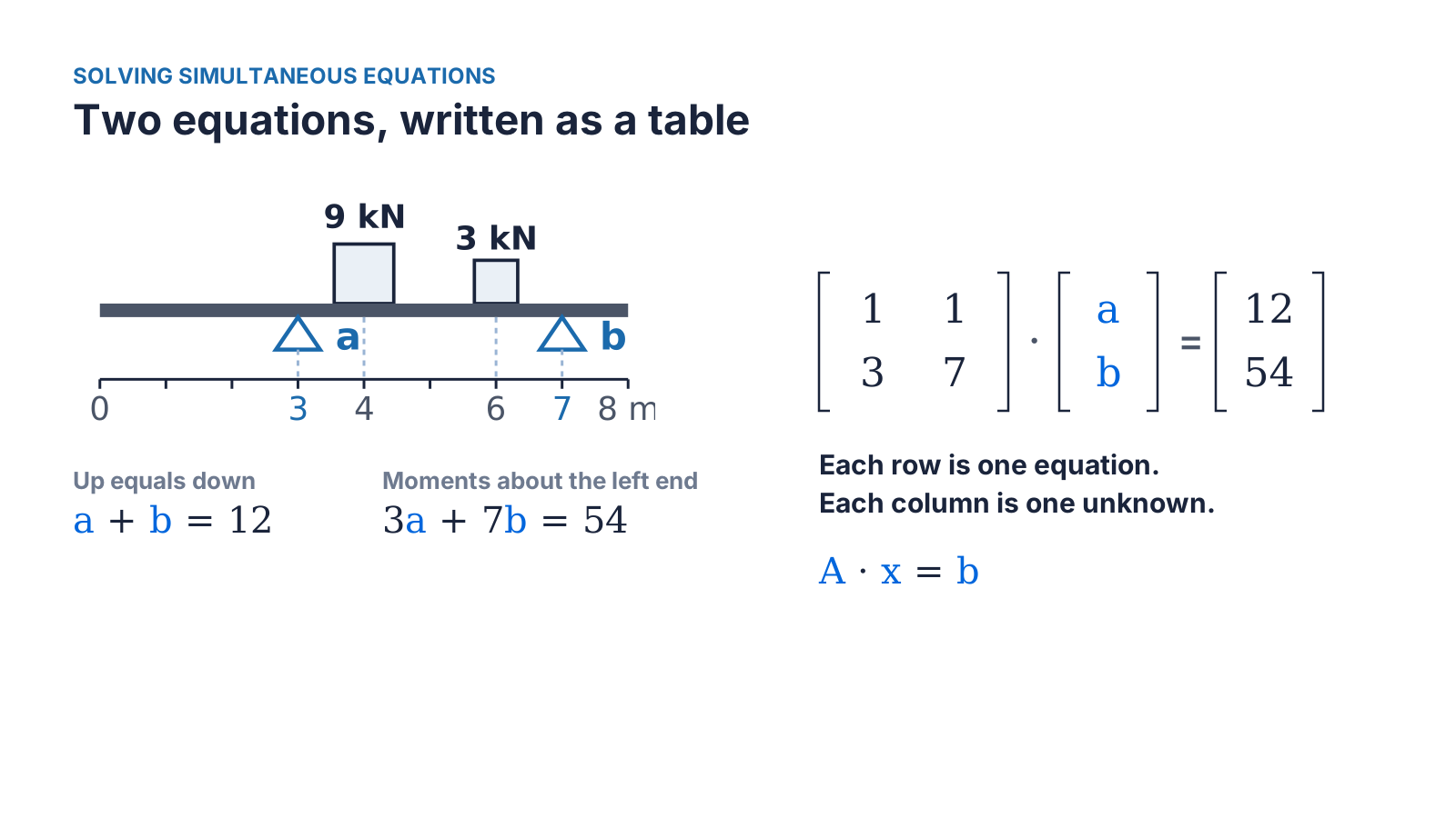
Lifting out the numbers in front of a and b gives a 2 × 2 matrix A with rows (1, 1) and (3, 7), and the loads give the vector b = (12, 54). Multiplying A by the unknowns gives back both equations: 1 × a + 1 × b in the first row, 3 × a + 7 × b in the second. Nothing has been solved yet. The equations have only been tidied into a table.
How a solver finds the answer
Solving A·x = b is the elimination method taught at school, carried out in a fixed order. Write the loads beside the matrix. Subtract three times row 1 from row 2, which removes a from the second equation and leaves 4b = 18. Divide row 2 by 4 to get b = 4.5. Subtract row 2 from row 1 to get a = 7.5. Once the left-hand block has ones on the diagonal and zeros elsewhere, the right-hand column is the answer.
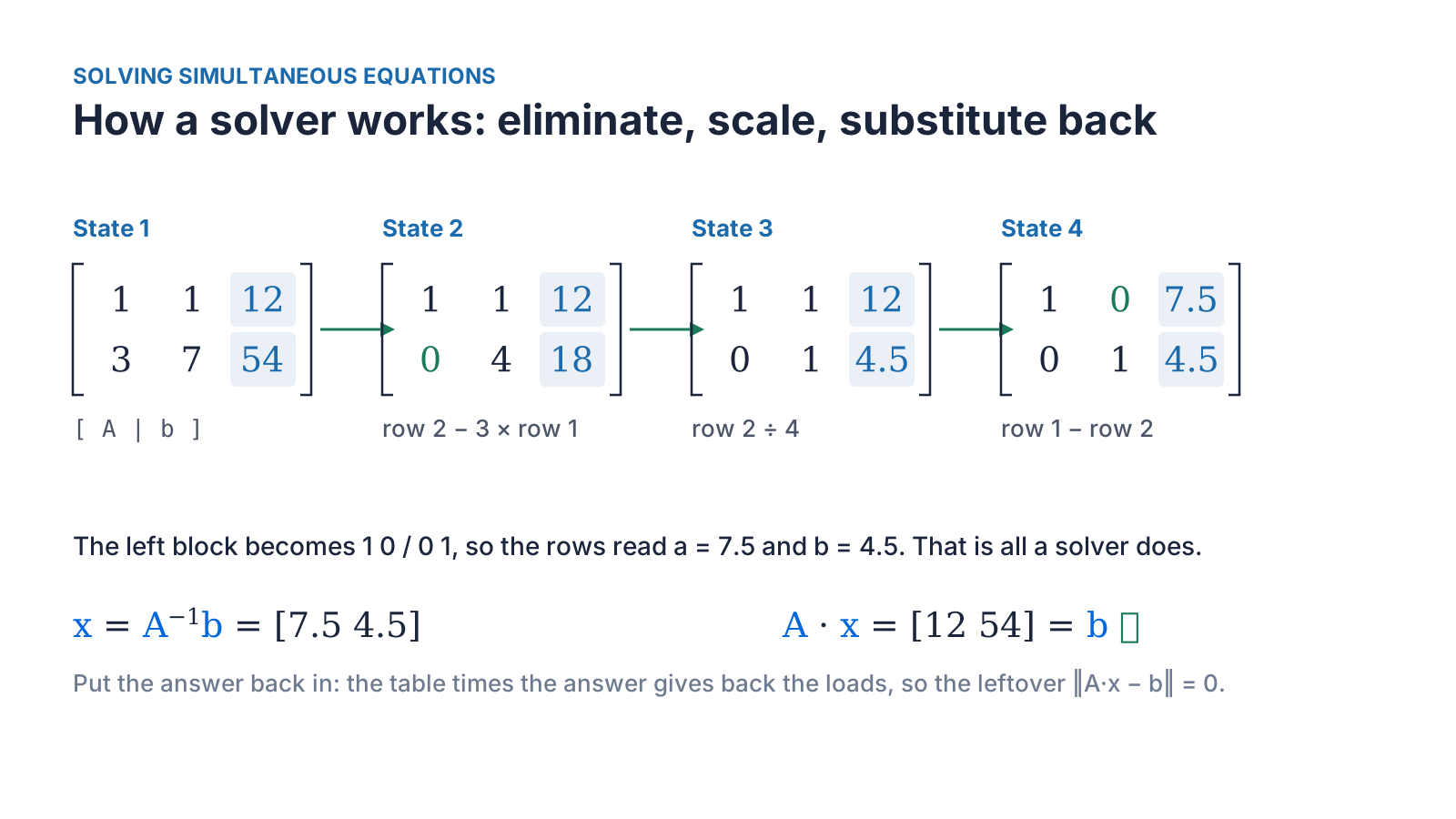
Every equation solver, from a spreadsheet to an FE package, follows this same pattern of eliminating, scaling and substituting back. That is why the method doesn't change when the matrix grows from two rows to two hundred thousand. Only the bookkeeping gets bigger.
The inverse and the determinant
The matrix that undoes A is its inverse, A⁻¹, defined so that A⁻¹·A gives the identity matrix: ones on the diagonal and zeros elsewhere, the matrix version of the number 1. For the plank, A⁻¹ is one quarter of the matrix with rows (7, −1) and (−3, 1), and x = A⁻¹·b gives the same 7.5 kN and 4.5 kN. Solvers rarely calculate the inverse itself, because solving directly is quicker and more accurate, but the idea is worth knowing.
The 4 in that quarter is the determinant of A: 1 × 7 − 1 × 3 = 4. The determinant is a single number that tells you whether the equations have one answer. If it is zero, they don't. Put both props at 3 m and the second row becomes three times the first, the determinant becomes zero, and no amount of algebra will separate the two reactions.
Checking the answer
Always put the answer back in. Multiply A by the answer and subtract the loads. What is left, one number per equation, is the residual, and for the plank it is zero in both rows. For a large problem the residual is summarised by its length, ‖A·x − b‖: square each leftover, add them up and take the square root. Because each leftover is squared, a +5 in one equation can't cancel a −5 in another, so a result near zero really does mean that every equation balances.
Keeping units consistent
Each row of a matrix can carry its own units, as long as every term in that row agrees. In the plank the first row is in kN and the second in kN·m. In a large matrix, though, moment rows can hold numbers hundreds of times bigger than force rows. Dividing the moment rows by a characteristic length, such as the typical distance between supports, brings them to a similar size, so rounding errors aren't concentrated in the largest values.
Solving many load cases at once
In A·x = b, the matrix A depends only on the geometry and the supports. The loads appear only in b. So a structure with many load cases needs only one matrix: put each load case in its own column of a load matrix B, and solving A·X = B returns one column of results for each case.
One plank, three load cases
1
- Loads
- 9 kN at 4 m and 3 kN at 6 m
- Reaction a (kN)
- 7.5
- Reaction b (kN)
- 4.5
2
- Loads
- 12 kN at 2 m
- Reaction a (kN)
- 15.0
- Reaction b (kN)
- −3.0 (uplift)
3
- Loads
- 6 kN at 5 m
- Reaction a (kN)
- 3.0
- Reaction b (kN)
- 3.0
| Load case | Loads | Reaction a (kN) | Reaction b (kN) |
|---|---|---|---|
| 1 | 9 kN at 4 m and 3 kN at 6 m | 7.5 | 4.5 |
| 2 | 12 kN at 2 m | 15.0 | −3.0 (uplift) |
| 3 | 6 kN at 5 m | 3.0 | 3.0 |
The second case shows the value of solving systematically: a load outside the props lifts the far prop, and the negative reaction flags it straight away. The same approach scales up. Cargo on a ship's deck can accelerate forward or aft, to port or starboard, and up or down, under roll, pitch and quartering seas: 24 load cases, one matrix, and 24 columns of loads.
Beams analysed with Macaulay's method are another good fit. Integrating the step and ramp terms leaves several constants of integration, one for each boundary condition. Writing one equation per boundary condition and solving them together gives every constant in one step, however many supports and loads the beam has.
Checking a structure is stable
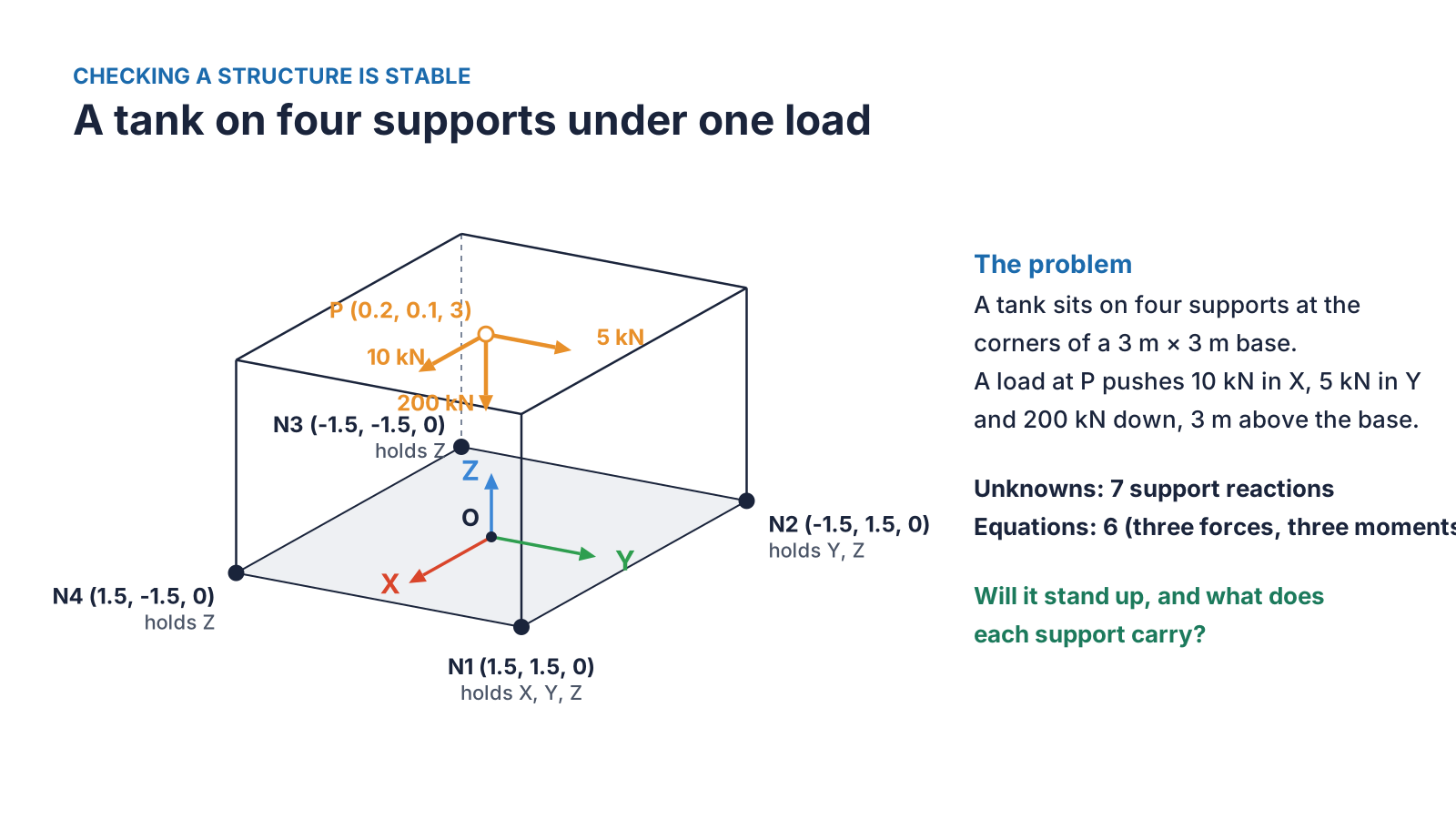
Here is a typical support problem. A tank sits on four supports at the corners of a 3 m square base. A load at P, 3 m above the base, pushes 10 kN in X, 5 kN in Y and 200 kN downwards. Support N1 is held in all three directions, N2 in Y and Z, and N3 and N4 only vertically. Will it stand up, and what does each support carry?
Writing the equilibrium equations
A rigid body in three dimensions has six equations of equilibrium. The forces in X, Y and Z must each add up to zero, and so must the moments about the X, Y and Z axes. Each restrained direction at a support is one unknown reaction, so this tank has seven unknowns: three at N1, two at N2 and one each at N3 and N4.
Each reaction gets its own column in the matrix. A force appears in its own force row, with a 1, and in the moment rows through its lever arm. A vertical reaction at a support 1.5 m from the X axis contributes 1.5 to the moment about X, exactly as you would write it by hand. The pattern of ones and lever arms is the cross product, r × F, written out as a table.
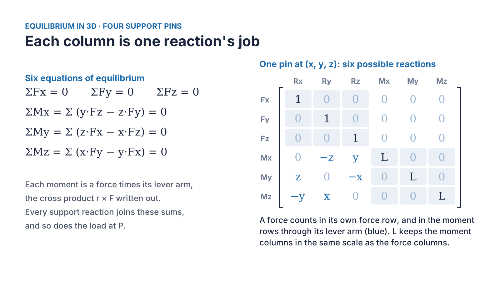
Writing every support the same way, with all six possible columns, and then switching off the directions that aren't held, means one layout handles any support arrangement. A roller, a pin and a fully fixed base differ only in which columns are kept.
Rank: are there enough independent equations?
Before solving, check the rank. The rank of a matrix is the number of its rows that are genuinely independent, that say something the others don't. The equations x + y = 2 and 2x + 2y = 4 look like two equations but are one, so their matrix has rank 1. For supports in 3D the matrix needs rank 6: all six equilibrium equations must be resisted by something. With anything less the structure is a mechanism, free to slide or spin, however reasonable the numbers look.
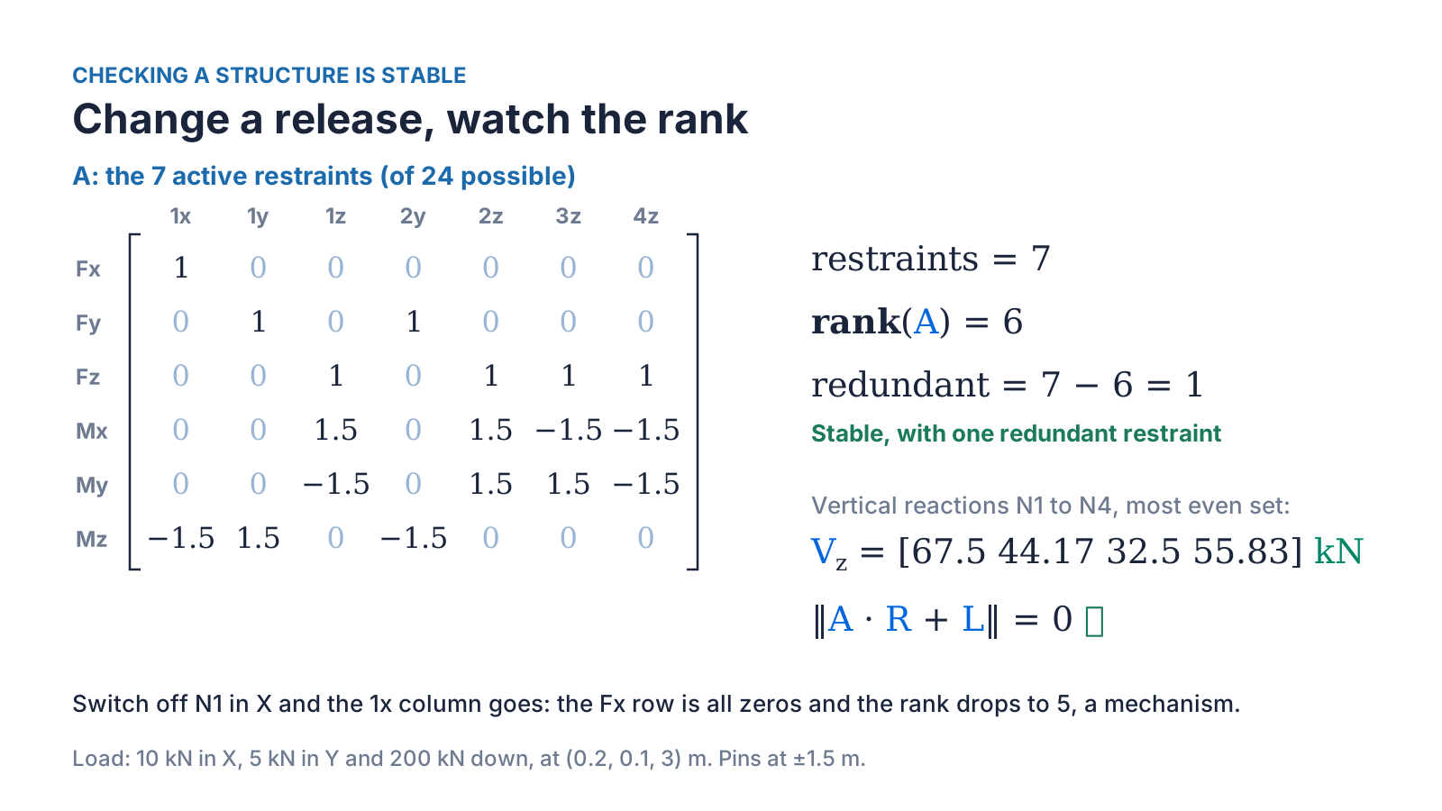
For the tank, the seven restraints give rank 6, so it is stable, and 7 − 6 = 1 restraint is redundant. Statics alone can't split the load between redundant supports, so the calculation takes the most even set of reactions that balances, explained in the next section. The vertical reactions come out at 67.5, 44.17, 32.5 and 55.83 kN, adding up to the 200 kN load, and the residual is zero.
Changing the supports changes only which columns are kept, so the same calculation checks every arrangement:
Change a release, watch the rank
N1 XYZ, N2 YZ, N3 Z, N4 Z
- Rank
- 6
- What it means
- Stable, 1 redundant
- Vertical N1 / N2 / N3 / N4 (kN)
- 67.5 / 44.17 / 32.5 / 55.83
The same, with N4 removed
- Rank
- 6
- What it means
- Determinate, no redundancy
- Vertical N1 / N2 / N3 / N4 (kN)
- 123.3 / −11.7 (uplift) / 88.3 / 0
All four supports XYZ
- Rank
- 6
- What it means
- Stable, 6 redundant
- Vertical N1 / N2 / N3 / N4 (kN)
- 67.5 / 44.17 / 32.5 / 55.83
Nothing resisting X
- Rank
- 5
- What it means
- Mechanism: no answer
- Vertical N1 / N2 / N3 / N4 (kN)
- None, by design
| Fixed directions | Rank | What it means | Vertical N1 / N2 / N3 / N4 (kN) |
|---|---|---|---|
| N1 XYZ, N2 YZ, N3 Z, N4 Z | 6 | Stable, 1 redundant | 67.5 / 44.17 / 32.5 / 55.83 |
| The same, with N4 removed | 6 | Determinate, no redundancy | 123.3 / −11.7 (uplift) / 88.3 / 0 |
| All four supports XYZ | 6 | Stable, 6 redundant | 67.5 / 44.17 / 32.5 / 55.83 |
| Nothing resisting X | 5 | Mechanism: no answer | None, by design |
Removing N4 leaves exactly six restraints, so the structure is statically determinate, and the matrix shows N2 lifting off with −11.7 kN. Removing the X restraint at N1 leaves nothing to resist the 10 kN horizontal load: the X force row of the matrix is all zeros, the rank drops to 5, and there is no answer to find. A solver that returned numbers here would be wrong. That is why the rank check belongs inside the calculation rather than in the engineer's memory.
The habit worth adopting: count the restraints and check the rank before solving, then check the residual after.
Sharing load between redundant supports
A four-point lift is the classic redundant problem. A 100 kN load is lifted from four points at the corners of a 4 m by 2 m rectangle, with its centre of gravity 0.4 m and 0.2 m off centre towards sling 1. There are four unknown tensions but only three equations: vertical equilibrium, and moments about the two horizontal axes. Statics alone gives infinitely many sets of tensions that balance the load. It is the same reason a four-legged table rocks.
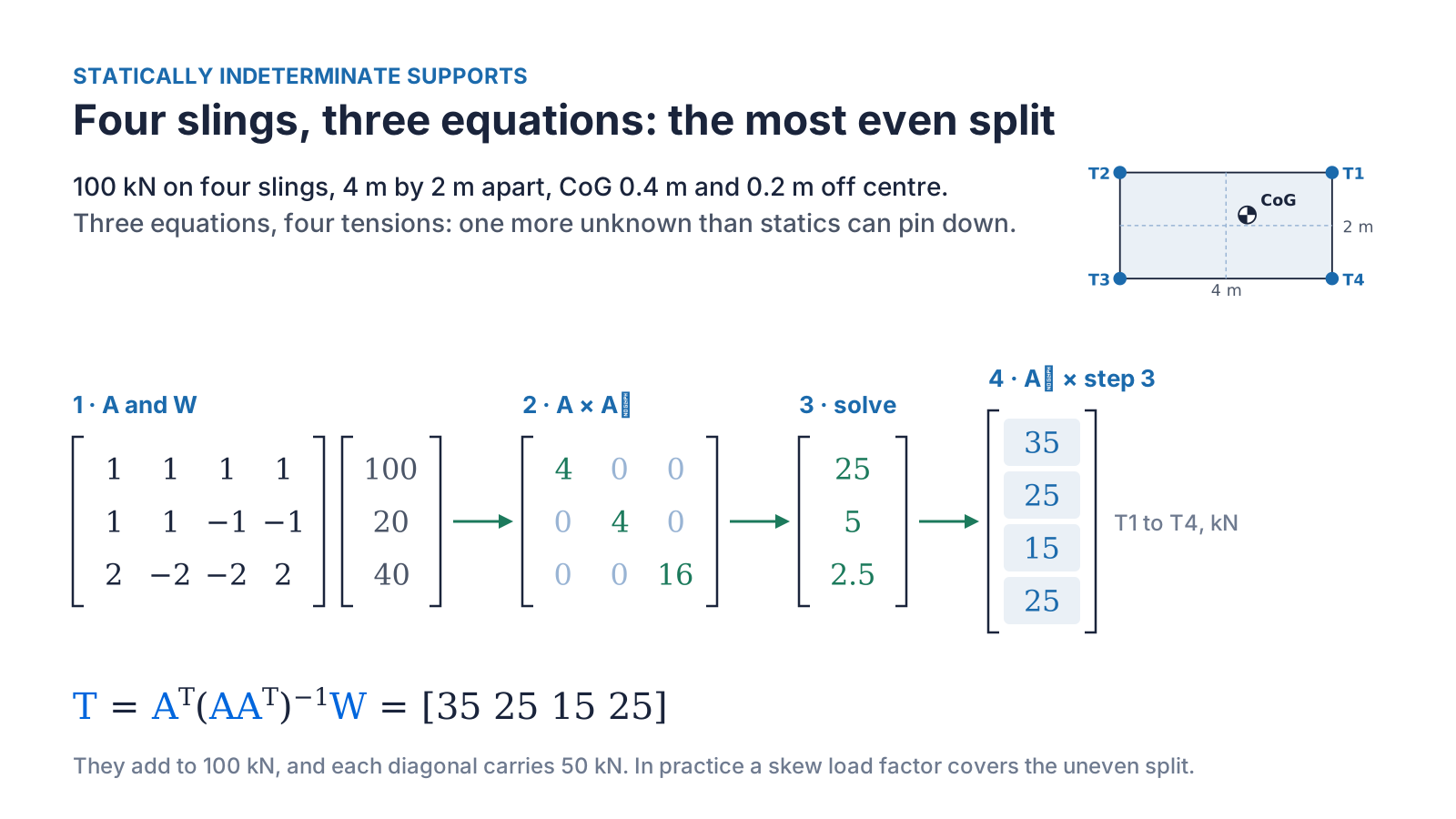
The matrix A is 3 × 4, so it has no inverse. Multiplying it by its own transpose Aᵀ, the same matrix with rows and columns swapped, gives a square 3 × 3 matrix that can be solved. Multiplying that result by Aᵀ turns three numbers back into four tensions. Written out, T = Aᵀ(AAᵀ)⁻¹W. This is the minimum norm solution: of all the sets of tensions that balance the load, it is the one with the smallest sum of squares, in other words the most even.
Here it gives 35, 25, 15 and 25 kN. They add up to 100 kN, sling 1 is the busiest and sling 3 the least loaded, and each diagonal pair carries 50 kN. In reality, slings of slightly different lengths or stiffnesses push the load onto one diagonal, which is why lifting design applies a skew load factor. The alternative is to include the sling stiffnesses, which gives a fourth equation and makes the problem determinate.
Resolving stresses to find principal stresses
Stress at a point in a material is itself a matrix: the direct stresses σx and σy on the diagonal, and the shear stress τ off it. Rotate the axes and all three numbers change, even though the material and the loading haven't. At one particular angle the shear stress disappears. The direct stresses at that angle are the principal stresses, the largest and smallest direct stresses at that point.
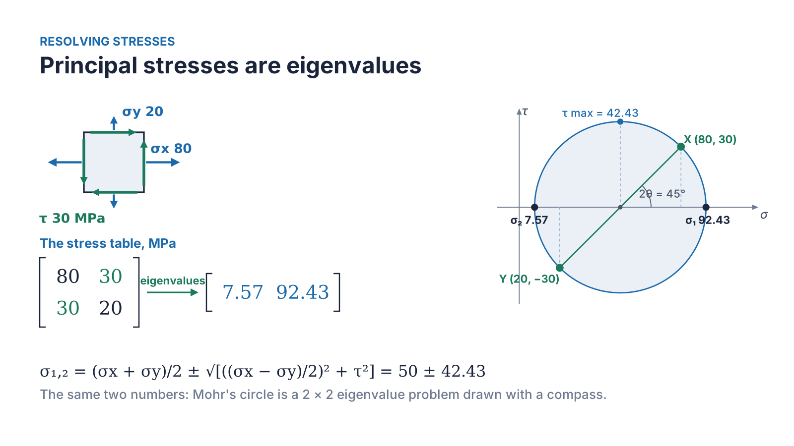
Finding that angle is an eigenvalue problem. An eigenvector of a matrix is a direction that the matrix only stretches, without turning, and its eigenvalue is the amount of stretch. For a stress matrix the eigenvectors are the principal directions and the eigenvalues are the principal stresses. They come from setting the determinant of (S − λI) to zero, where I is the identity matrix. For σx = 80 MPa, σy = 20 MPa and τ = 30 MPa this gives λ² − 100λ + 700 = 0, which is the familiar formula:
σ₁,₂ = (σx + σy)/2 ± √[((σx − σy)/2)² + τ²] = 50 ± 42.43, so σ₁ = 92.43 MPa and σ₂ = 7.57 MPa.
The principal directions are at 22.5° to the original axes, half the 45° angle on Mohr's circle, which is the same eigenvalue problem drawn with a compass. Notice that the maximum principal stress is higher than either direct stress you started with. That is why strength checks use principal stresses, or an equivalent stress built from them such as von Mises, rather than the raw components. In three dimensions the stress matrix is 3 × 3 and gives three principal stresses in the same way, which is what an FEA package calculates at every point when it plots principal or von Mises stress.
Creating a stiffness matrix for FEA
Finite element analysis solves one equation, F = K·d. F holds the forces at every node, d the displacements, and K is the stiffness matrix, which links every force to every displacement. It is Hooke's law, force equals stiffness times stretch, written for a whole structure at once.
Starting with two springs
Two springs in a line show how K is built. Spring 1, with a stiffness of 100 kN/m, joins a fixed node 1 to node 2. Spring 2, with a stiffness of 50 kN/m, joins node 2 to node 3. On its own, each spring has a 2 × 2 stiffness matrix with k on the diagonal and −k off it: pull one end and the spring resists at that end and pulls on the other.
Adding both springs into a 3 × 3 matrix, at the nodes they connect, gives rows of (100, −100, 0), (−100, 150, −50) and (0, −50, 50) kN/m. Node 2 is shared, so its diagonal term is the sum of both springs, 100 + 50 = 150 kN/m. Node 1 is fixed, so its row and column are removed. Applying 10 kN at node 3 and solving the remaining 2 × 2 equations gives displacements of 0.1 m at node 2 and 0.3 m at node 3. Putting those back into the removed row gives the reaction at node 1, 10 kN, balancing the load.
That is the whole method: build each element, assemble them at the shared nodes, remove the held directions, solve for the displacements, then recover the reactions.
Beams and frames
Real members stretch, bend and rotate, so each end of a 2D frame member has three movements and the member's stiffness matrix is 6 × 6. It is easiest to write in the member's own axes, along and across it. A member on a slope is rotated into the global axes with K_G = Tᵀ k T, where T is the rotation matrix built from the cosine and sine of the member's angle. Read it from right to left: rotate the movements into the member's axes, apply the simple stiffness, then rotate the forces back.
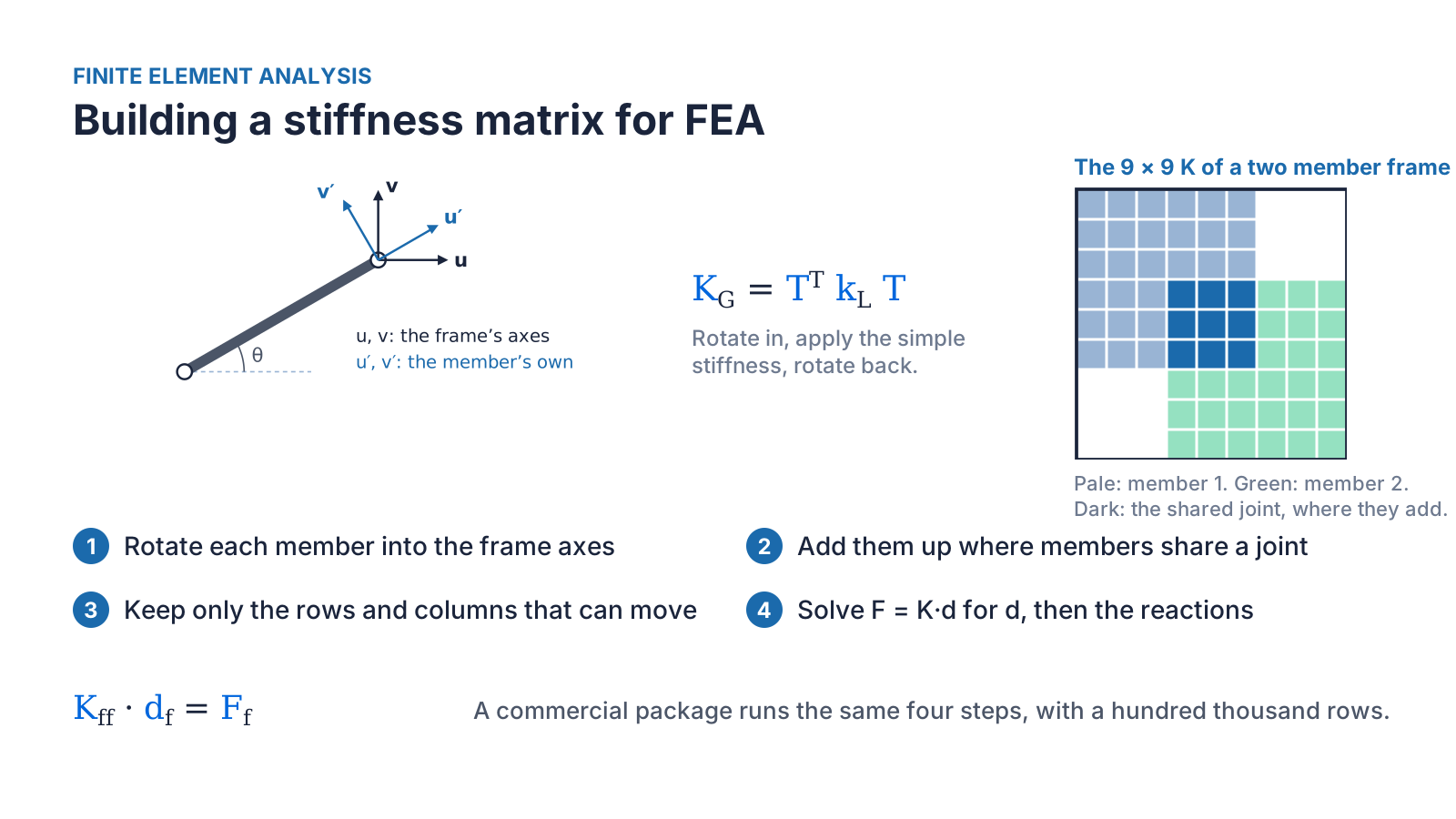
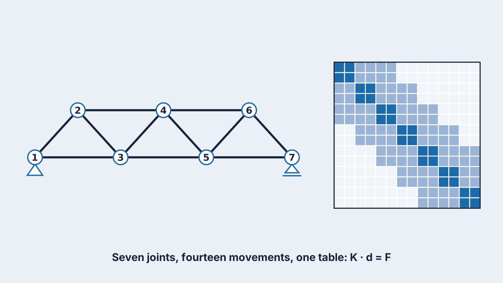
Each rotated member is added into the global matrix at the joints it connects, exactly like the springs, and where members share a joint their stiffnesses add. The held rows and columns are removed, the free displacements are solved for, and the reactions follow. The truss stiffness matrix at the top of this post shows the result: a dark block on the diagonal for each joint, a pale block for each member joining two joints, and zeros everywhere else. Most of a real stiffness matrix is zeros, which is what lets FE solvers handle millions of unknowns. A commercial package runs these same steps, with more sophisticated elements and far more rows.
More problems matrices solve
- Natural frequencies and mode shapes: solving (K − ω²M)·φ = 0, an eigenvalue problem built from the stiffness and mass matrices, gives the frequencies at which a structure wants to vibrate. Vibration checks on machinery skids, masts and offshore structures start here.
- Buckling loads: the eigenvalues of the stiffness and geometric stiffness matrices give the load factors at which a frame or plate buckles, and the eigenvectors give the buckled shapes.
- Fitting test data: with more measurements than unknowns, least squares finds the line or curve that fits best. It uses the transpose in a similar way to the four-point lift.
- Pipe, hydraulic and electrical networks: one equation per junction for flow and one per loop for pressure or voltage, solved together.
- Coordinate transformations: rotation matrices move loads, positions and accelerations between body and global axes, for crane slewing, vessel motions and robot arms.
- Heat transfer and seepage: a grid of nodes gives a large, sparse set of equations with the same structure as a stiffness matrix.
Good practice
- Count the unknowns and the equations, and check the rank, before you solve.
- Check the residual after you solve, and after any transformation.
- Keep the units consistent along each row.
- Use one global coordinate system and one moment sign convention (the right-hand rule), with every position measured from one reference point. Reactions then come out with the correct sign, without guessing their direction first.
- Solve rather than invert: solving A·x = b directly is faster and more accurate than calculating A⁻¹.
The operations behind all of this
Multiply A·x
- What it tells you
- Turns unknowns into equation results
- Where you meet it
- Writing equations; checking an answer
Solve A·x = b
- What it tells you
- The unknowns
- Where you meet it
- Reactions, displacements, member forces
Transpose Aᵀ
- What it tells you
- Rows and columns swapped
- Where you meet it
- Rotating members; sharing load between redundant supports
Inverse A⁻¹
- What it tells you
- The matrix that undoes A
- Where you meet it
- Theory and flexibility matrices; rarely calculated directly
Determinant
- What it tells you
- Zero means there is no single answer
- Where you meet it
- A quick check before solving; characteristic equations
Rank
- What it tells you
- How many independent equations there are
- Where you meet it
- Stability and mechanism checks
Norm ‖v‖
- What it tells you
- The size of a list as one number
- Where you meet it
- Residual checks
Eigenvalues and eigenvectors
- What it tells you
- Directions a matrix only stretches, and by how much
- Where you meet it
- Principal stresses, natural frequencies, buckling
| Operation | What it tells you | Where you meet it |
|---|---|---|
| Multiply A·x | Turns unknowns into equation results | Writing equations; checking an answer |
| Solve A·x = b | The unknowns | Reactions, displacements, member forces |
| Transpose Aᵀ | Rows and columns swapped | Rotating members; sharing load between redundant supports |
| Inverse A⁻¹ | The matrix that undoes A | Theory and flexibility matrices; rarely calculated directly |
| Determinant | Zero means there is no single answer | A quick check before solving; characteristic equations |
| Rank | How many independent equations there are | Stability and mechanism checks |
| Norm ‖v‖ | The size of a list as one number | Residual checks |
| Eigenvalues and eigenvectors | Directions a matrix only stretches, and by how much | Principal stresses, natural frequencies, buckling |
None of this replaces engineering judgement. What matrices add is a reliable way to write the equations once, solve them for every case, and prove that the answer balances. Spreadsheets, MATLAB, Python and every FE package work this way. At Subco we build these methods and checks into our in-house calculation tools, so repeated load cases and support checks are done the same way every time.
Category:
Blog
Written by:

Martin Reynolds